When analyzing large amounts of data, we are often interested in trends and correlations. One of the most basic methods to research these, is linear regression. Linear regression is a statistical method to determine the correlation between different variables in a data set. New DAX functions have been introduced recently, that provide linear regression capabilities. In this blog post, we dive into these new functions: LINEST and LINESTX.
To illustrate the concept of linear regression, I have loaded a data set of cars in the Netherlands. Many details of vehicles are available through open data sets. The prices of registered vehicles are available for about 8 million vehicles registered since 2004 which are still on the road. The chart below shows the average vehicle price by year of registration. I have added a trend line through the analysis options of the column chart:
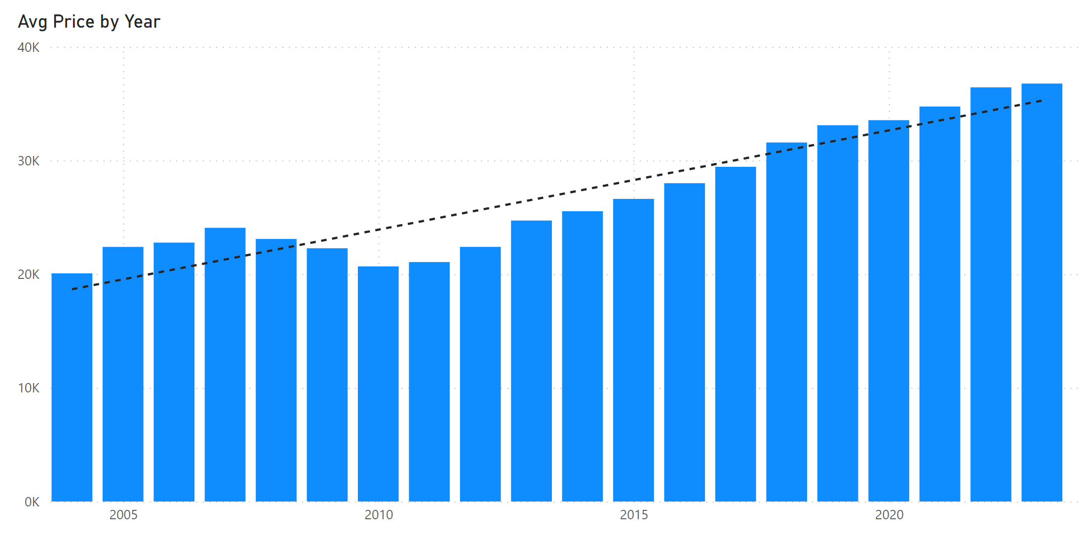
The trend line gives a rough indication of the growth in the average price over the years. It is determined through simple linear regression on one variable; in this case, the year.
In mathematical terms, the challenge in linear regression is to find, for a collection of (x,y) pairs, a function
![]()
such that the line defined by this function is ‘closest’ to the collection of (x, y) pairs. The common way to find the function is through the ‘least squares’ method, which comes down to determine values for a and b for which the total error is smallest. That is, for each (x, y) pair, there is a difference between y and F(x): the error. F(x) could be larger or smaller than y; this problem is solved by working with the quadratic form: (F(x) – y)2.
For simple linear regression, exact mathematical expressions exist for the a and b values. This means that it can be solved with DAX in any Power BI model. In our book Extreme DAX, we describe how this can be done. When you want to do linear regression on more than one variable, things become complicated: the only thing possible is to use some algorithm to approximate the F(x) function.
The new DAX functions LINEST and LINESTX do exactly that. This means that we now have easy-to-use functions to do linear regression in Power BI. I will demonstrate this using the simple data model containing vehicle registrations:
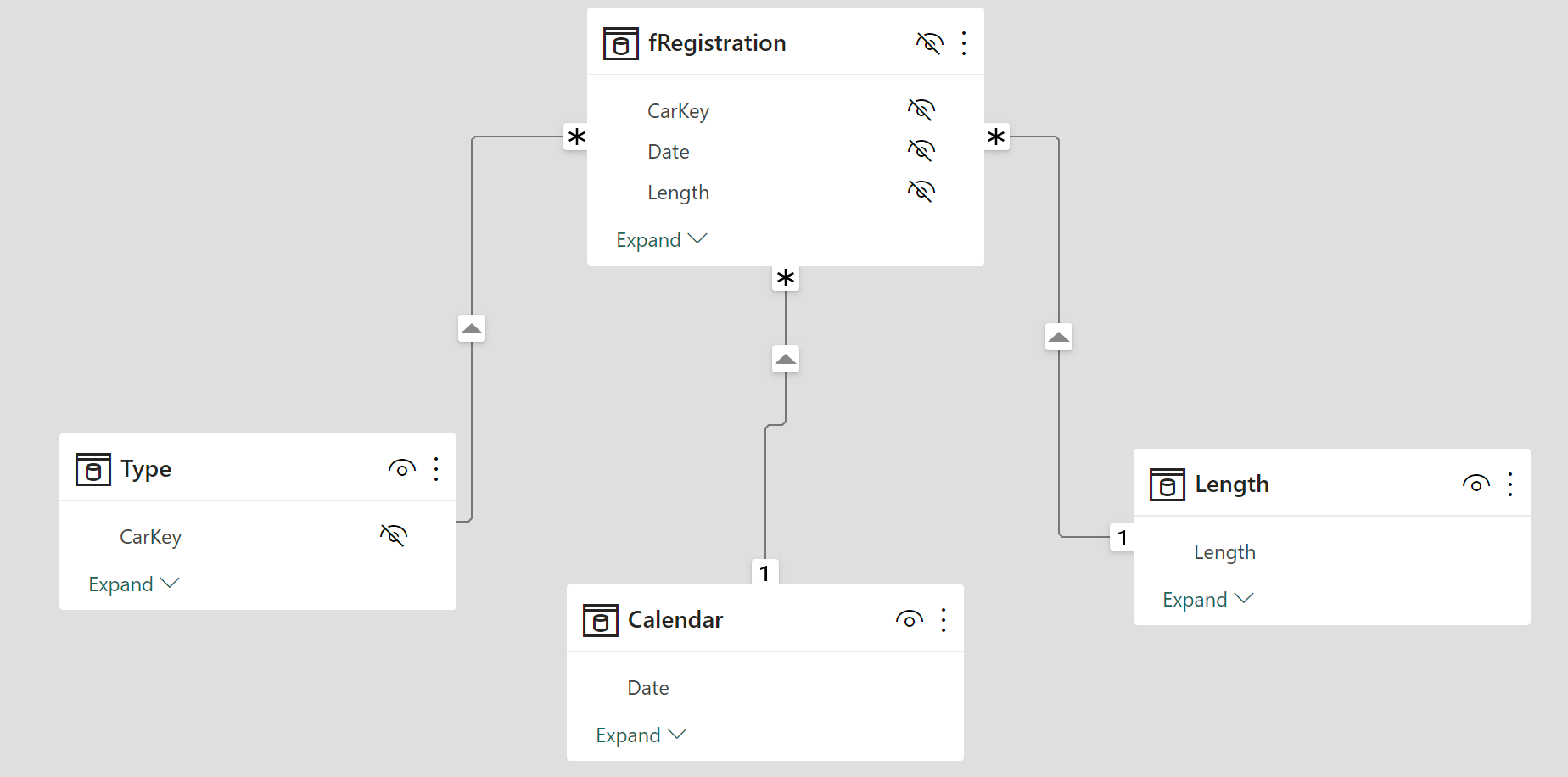
The LINEST and LINESTX functions need the data points, the (x, y) pairs, and have a unique form of output which is a first for DAX. Logically, the output would be the function F; but DAX cannot do that at the moment. Instead, a one-row table is returned containing the building blocks for F together with additional information about the linear regression. You can use the data in the table to build the F function yourself.
I prefer to use the LINESTX function, as this gives you ultimate control on the data points used. LINESTX takes a table as its first argument, of which each row will define a data point to do linear regression on. The second argument must provide the y value for each data point. Other arguments provide x values. To start with simple linear regression on the year, I’ve created a calculated table using the formula below:
Est Price (Year) =
LINESTX(
DISTINCT(‘Calendar'[Year]),
CALCULATE(AVERAGE(fRegistration[Price])),
‘Calendar'[Year]
)
The formula takes the different values for Year from the Calendar table, calculates the average price for vehicles for each year (the y values) and the years themselves (the x values). The result is this table (shortened for readability):

The columns Slope1 and Intercept are the important ones to build the F function. In our mathematical formula used earlier, a corresponds to Slope1 while b is the Intercept. A DAX measure to calculate the regression line can be created like this:
Price (Regression Year) =
VAR ThisYear = SELECTEDVALUE(‘Calendar'[Year])
VAR Intercept = MIN(‘Est Price (Year)'[Intercept])
VAR Slope = MIN(‘Est Price (Year)'[Slope1])
RETURN
Slope * ThisYear + Intercept
The result is similar to the trendline, but now, of course, we can use the measure to estimate the average price for, say, 2024.
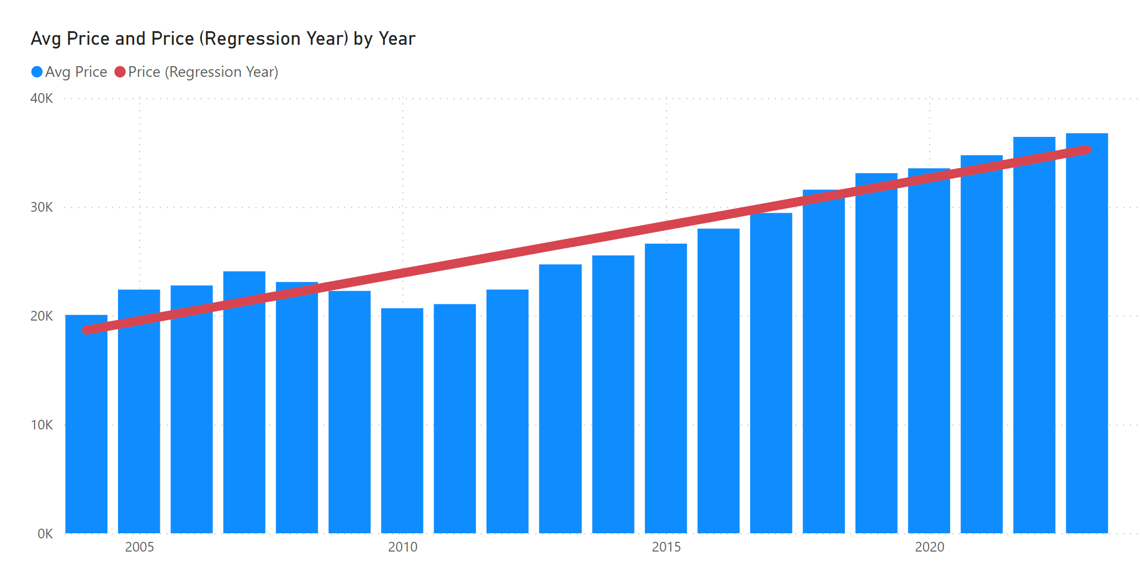
Obviously, taking only the year as variable to estimate the vehicle price will result in a very rough estimate. That is why it is interesting to add more variables. For instance, the formula below takes the length of a vehicle into account as well:
Est Price 2 =
LINESTX(
SUMMARIZE(fRegistration, ‘Calendar'[Year], Length[Length]),
CALCULATE(AVERAGE(fRegistration[Price])),
‘Calendar'[Year],
Length[Length]
)
This time, we use SUMMARIZE to retrieve all unique combinations of year and vehicle length as the base table. Be careful with this: the LINESTX function can take a lot of time calculating when you feed it with a very large number of data points. You may consider, for instance, to first create some buckets of length ranges and use these instead of each unique vehicle length. The result looks like this:

As we now have two x variables, year and length, we have two Slope values as well. The measure to compute the estimation is:
Price (Regression Year – Length) =
VAR ThisYear = SELECTEDVALUE(‘Calendar'[Year])
VAR ThisLength = SELECTEDVALUE(Length[Length])
VAR Intercept = MIN(‘Est Price 2′[Intercept])
VAR SlopeYear = MIN(‘Est Price 2′[Slope1])
VAR SlopeLength = MIN(‘Est Price 2′[Slope2])
RETURN
SlopeYear * ThisYear + SlopeLength * ThisLength + Intercept
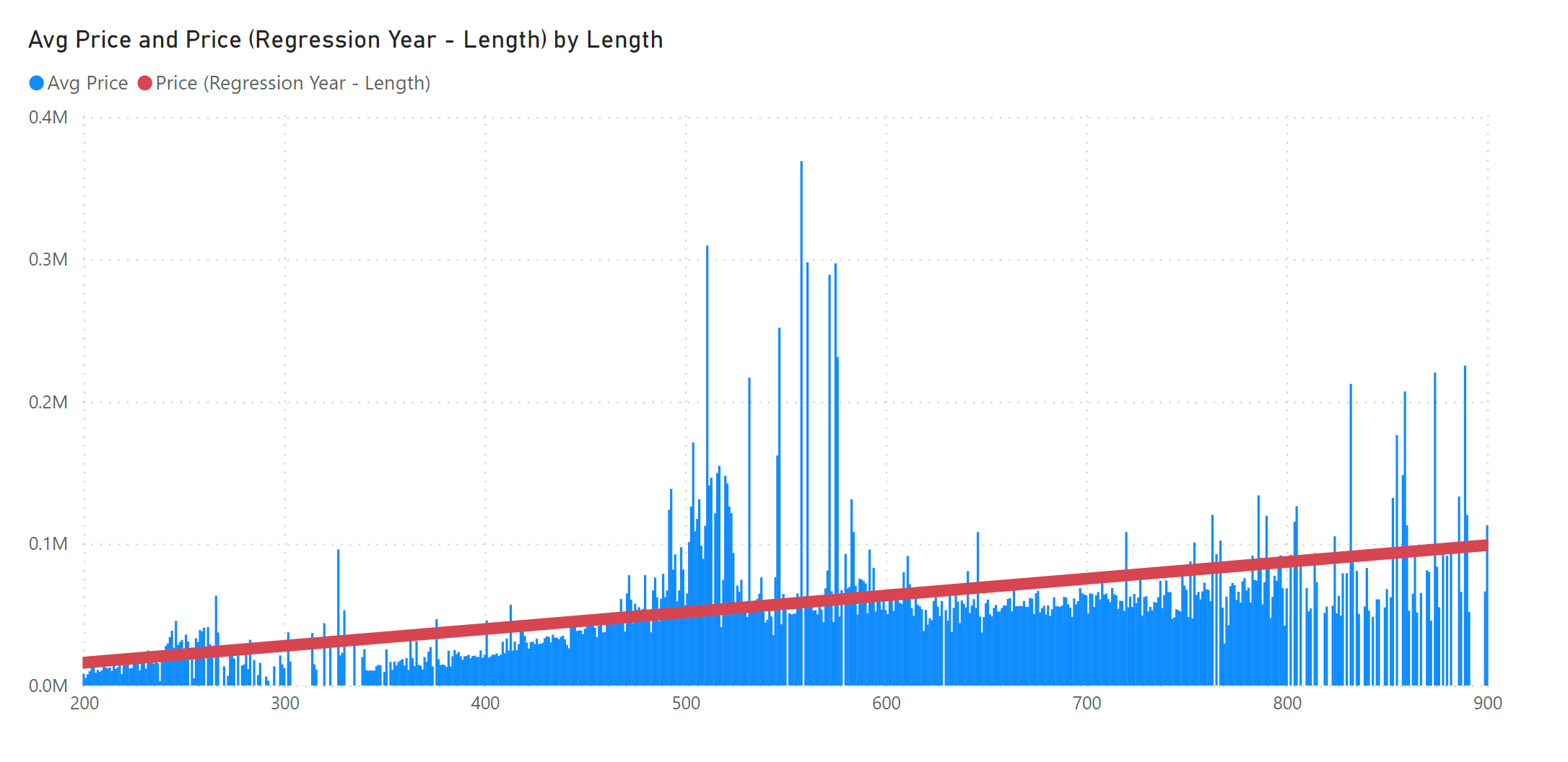
This defines a function that would look great in a 3D chart, but can also be visualized with standard visuals and filters. Below is the regression line on vehicle length for the year 2021:
A common misunderstanding is that linear regression will always result in a straight line. The linear aspect of linear regression is that we assume a linear relationship between the function F and its input variables. But nothing keeps us from using nonlinear input variables! You may have noticed that the actual average price over the years does not particularly look like a straight line. Below, we use LINESTX with the year and the square of the year as input:
Est Price X2 =
LINESTX(
ADDCOLUMNS(
DISTINCT(‘Calendar'[Year]),
“X2”, ‘Calendar'[Year] ^ 2
),
CALCULATE(AVERAGE(fRegistration[Price])),
‘Calendar'[Year],
[X2]
)
The corresponding DAX measure must use the square of the year as well, of course:
Price (Regression X2) =
VAR ThisYear = SELECTEDVALUE(‘Calendar'[Year])
VAR Intercept = MIN(‘Est Price X2′[Intercept])
VAR SlopeX = MIN(‘Est Price X2′[Slope1])
VAR SlopeX2 = MIN(‘Est Price X2′[Slope2])
RETURN
SlopeX * ThisYear + SlopeX2 * ThisYear ^ 2 + Intercept
The result of this linear regression looks like this:

When doing linear regression, which variables to use is an important choice to make. While doing this, you slowly enter into proper data science territory, in which you will want to make informed decisions on the variables to avoid overfitting, optimize for accuracy, et cetera. Nevertheless, the addition of LINEST and LINESTX is an exciting development in DAX!

