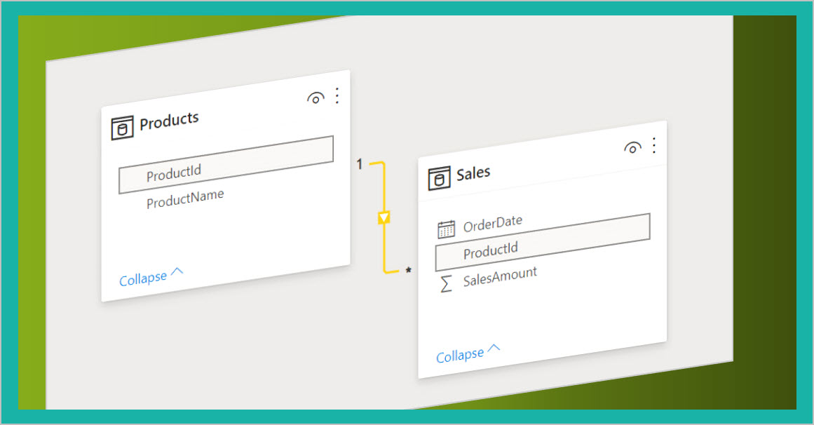
In this second blog about achieving a different mindset when you want to change business tools, I want to talk about the creating an extra numeric column as relation column between tables. If you want to know more about normalized tables, please read my first blog on this subject.
If you can connect to a relational database, within your Power BI model, most of the time there is no problem. Part of the table is a numeric column created with the special purpose for relationships. Add that column to your template of model and most of the time you are good to go. If you can adjust the import template to provide those columns, you certainly should do this!
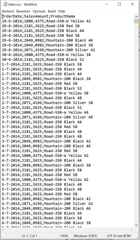
But not everyone has such a luxury position. If the only way to get your data by using a prepared templated download, without the possibility to download the original table, you need to take care of the creating a dimension (or filter) table, including the normalized, numeric column, yourself. We start from a sales table, stored in CSV format.
Note. Data from a template can retrieve and store data in different formats. The most popular download format is Excel. I recommend you start changing your download format to CSV or text format. If you realize that volume of data is not a problem within apps like Power BI or Power Pivot in Excel, you will prefer to make a report spanning several years and based on the lowest hierarchical level, in comparison to the one-year, compressed report in traditional Excel. If you use an Excel template you are restricted to 1.048.576 rows, while Text of CSV format does not have this limitation.
Now you have multiple options. If you want to create a dimension or filter table and adjust the fact table, you basically have two different ways: manual or automatic created tables. I will discuss both options, but in advance I will state that manual labor should always be avoided.
If you talk about manual creating a dimension table you can create the table in Excel or another program that can handle structured data, for instance a database-based application like Access or SharePoint list.
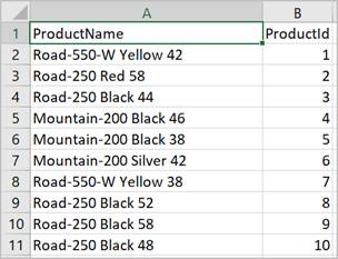
To create the dimension table, you can import the table in Excel en remove all columns, except the Column ProductName.
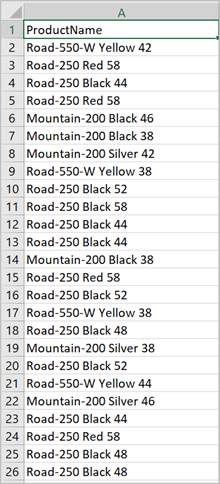
Next, you want this column contains unique values. You can perform this action manually, but with lots of data that is not a durable option. So, use the Remove duplicates option.


Type 1 in the column after the first data row and us the fill handle to copy a unique number to the table.
Now you can use a simple VLOOKUP to add the ProductID to the original fact table.
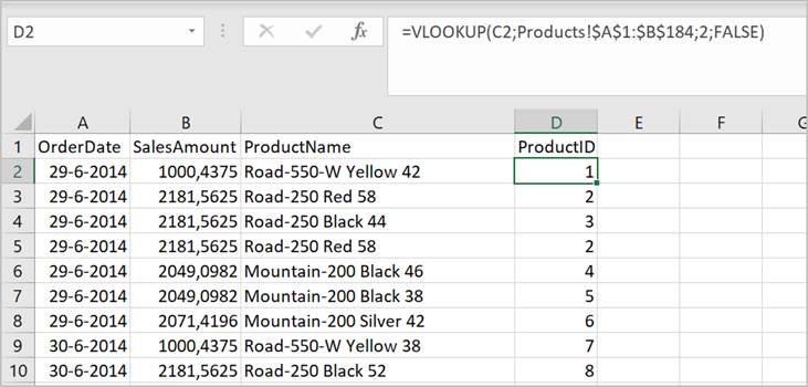
There are disadvantages to this method. First at all, manual interaction is the main source of errors since you need to repeat all actions in the same way each time you to do a refresh. Undoubtedly this option will cost you time compared to an automatic process. The second problem is that you would like to remove the column ProductName, since it is replaced by the PorductID. In Excel this is not possible, because the VLOOKUP calculation uses this column. All in all, you do not get anywhere with this method. The last problem has been stated before. If your fact has more the one million rows, the Excel sheet will be filled completely, ignoring the surplus of rows.
So, let us see how this can work, using Power Query in Power BI. You can achieve the same results in Power Query in Excel if you land the results in the Data model (Power Pivot) to avoid the problems with the one-million row problem.
I have opened the Sales.csv file in Power Query.

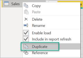
The next step is the make a duplicate of the table en rename the query in Products.
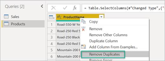
Now you select the column ProductName and Remove Other Columns.

Then Remove Duplicates.
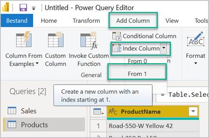
And finally add an Index column, starting from 1.
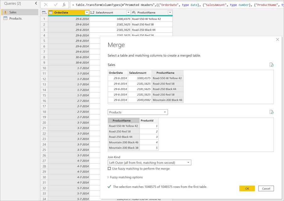
In the next steps you add the ProductId to the Sales table by using Merge Queries (Ribbon Start).
And expand the Products column.
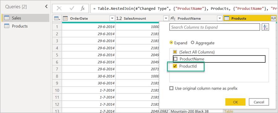
Since Power Query does not rely on calculations, you are perfectly able to remove the column ProductName.

You use the columns ProductId in both tables within the Data Model to create and use the relationship.
This method will be repeated, every time you perform a (manually or automatic) refresh. If you have multiple fact tables, you append the different fact tables into one table and then repeat the above-mentioned actions. There are also some minor disadvantaged. First you really do not have much control over the index number, since it will be renewed every refresh. Since you merge the number again in the refresh cycle, in which the number will be again applied. The other disadvantage can be the long waiting time when large fact tables are involved during refresh. But again, in the production stage (and there you want speed and no waiting time) a numeric type column will perform much faster in comparison of a text type column.
In my next blog I will discuss the differences in the storage of data. The choices I like to discuss are storing in (separate) Excel files, SharePoint (online) lists, Power BI models or in DataFlows.
